Ashley Madison is an online dating service, launched in 2001 and based in Canada. Its target groups are individuals who are married or in a relationship. Its motto is: "Life is short. Have an affair." On July 15 this year the news broke that hackers had stolen its customer data, including emails, names, home addresses, credidt card information, etc. The hackers demended the service to shut down or they would publish the data. On 22 July, the first data were released. When the company did not shut down, all customer data was released on 18 August. A final batch of data was released on 20 August 2015.

At the beginning the data was only available in the so called "dark web", but later it leaked to mainstream websites. The data released on 18th August, consisted of a dump of about 9-10 GB. It has been claimed that data of that size is difficult to analyse using standard computer hardware. In this post I will show how this data can be analysed and some conclusions can be drawn. I will abstain from disseminating any personal information as I do not want to contribute to destroying lives of those affected by the hack. I will not divulge credit card details or anything like that. I will also not explain in detail how to obtain the data dump; even thought that step has been explained in great detail on many websites. I will, however, show how to work with the data and show some potentially interesting aspects of it.

The following analysis was done together with Bjoern Schelter, who helped with the mySQL connection and who is also a member of this community. The first part of the post is a little bit dry. It explains how to connect to an mySQL database. I hope that the second part of the post makes up for the first part. It will contain information on the gender balance, and reveal some other hopefully interesting bits of information.

In order to analyse this large data set we will use mySQL. I am working on Mac OS X and there are very easy instructions found online of how to install mySQL. The basic steps are:

• Download mySQL from here.
• Install the program.

• Run the following terminal command in the terminal:

  sudo /usr/local/mysql/support-files/mysql.server start

• Generate a file called ~/.bash_profile if it does not yet exist.

  cd ; nano .bash_profile

• Copy this line

  export PATH="/usr/local/mysql/bin:$PATH"

into the file and save.

• Set the root password for mySQL (from the command line)

  /usr/local/mysql/bin/mysqladmin -u root password 'yourrootpasswordhere'

• Fix the mySQL socket error:

  sudo mkdir /var/mysql
  sudo ln -s /tmp/mysql.sock /var/mysql/mysql.sock

• Then create this file:

  sudo nano /Library/LaunchDaemons/com.mysql.mysql.plist

and copy this into it:

<!--?xml version="1.0" encoding="UTF-8"?-->
<plist version="1.0">
  <dict>
    <key>KeepAlive</key>
    <true />
    <key>Label</key>
    <string>com.mysql.mysqld</string>
    <key>ProgramArguments</key>
    <array>
      <string>/usr/local/mysql/bin/mysqld_safe</string>
      <string>--user=mysql</string>
    </array>        
  </dict>
</plist>

Then save.

• Execute in the shell:

  sudo chown root:wheel /Library/LaunchDaemons/com.mysql.mysql.plist
  sudo chmod 644 /Library/LaunchDaemons/com.mysql.mysql.plist
  sudo launchctl load -w /Library/LaunchDaemons/com.mysql.mysql.plist

Now mySQL is installed. We now prodeed to construct our database from the dump. We follow the instructions on this website. The folder you would get if you downloaded the dump is called dmps. It contains several zip files. After unzipping the folder should look like this:

Ok. Now we need to run the following commands as root user in mysql (after login in the terminal using "mysql -u root -p"):

CREATE DATABASE aminno;
CREATE DATABASE am;
CREATE USER 'am'@'localhost' IDENTIFIED BY 'loyaltyandfidelity';
GRANT ALL PRIVILEGES ON aminno.* TO 'am'@'localhost';
GRANT ALL PRIVILEGES ON am.* TO 'am'@'localhost';

The next step will take a while: we have to import the database as normal user.

$ mysql -D am -uam -ployaltyandfidelity < am_am.dump
$ mysql -D aminno -uam -ployaltyandfidelity < aminno_member.dump
$ mysql -D aminno -uam -ployaltyandfidelity < aminno_member_email.dump
$ mysql -D aminno -uam -ployaltyandfidelity < member_details.dump
$ mysql -D aminno -uam -ployaltyandfidelity < member_login.dump

Depending on your computer each if these will run for 4-10 hours. A solid state disk seems to make a huge difference here. While this is running you might already start analysing some of the other files. The file swappernetQAUser_Table.txt contains many password in plain text with no encryption. I believe that nowadays that would be considered bad practice when it comes to handling peoples' passwords.

swappernet = Import["/Users/thiel/Desktop/dmps/ashleymadisondump/swappernet_QA_User_Table.txt", "CSV"];
passwords = Select[swappernet, Length[#] > 3 &][[;; , 4]]; Grid[(Reverse@SortBy[Tally[passwords], #[[2]] &])[[1 ;; 25]], Frame -> All]

The resulting table contains surprisingly simple passwords. Some of the top passwords are inappropriate for this community, and do not further our understanding, so I have blurred them out. This is the result:

There are

Length[swappernet]
(*765607*)

765607 entries in the file and the numbers of really, really unsafe passwords is quite low, but the 200 or so most frequent passwords would unlock about 10% of the profiles. This is a bit shocking, particularly because the accounts contain sensitive information.

Let's move on to the main databases. We will start with the data base "am". Let's increase the heap space for Java a bit like so:

<< JLink`;
InstallJava[];
ReinstallJava[CommandLine -> "java", JVMArguments -> "-Xmx4096m"]

To connect to the database we need the following driver:

Needs["DatabaseLink`"];
JDBCDrivers["MySQL(Connector/J)"]

I found that the easiest way to connect to the database is to use the DatabaseExplorer:

DatabaseExplorer[]

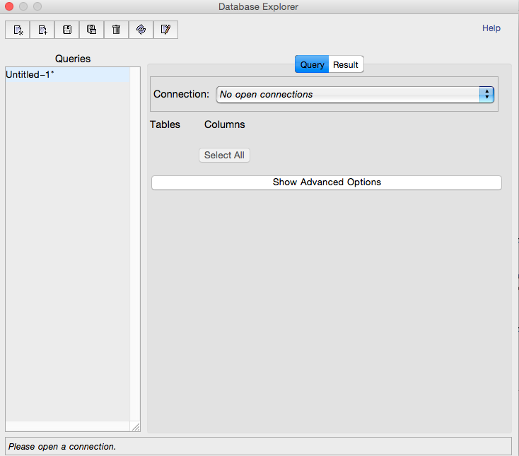
The interface is quite straight forward to use. You need to add a new database. You click on the first icaon ("add database") on the upper left and follow the instructions. You like the two databases we generated above "am" and "aminno". As "type of the databse" you use "MySQL(Connector/J)". The host is "localhost", and the password is "loyaltyandfidelity". Ok. Now we are ready to use Wolfram Language. Let's start with the am databse.

am = OpenSQLConnection["am", "Name" -> "am", "Password" -> "loyaltyandfidelity"]

So let's see what we've got:

colums = SQLExecute[SQLSelect["am", {"am_am_member"}, {SQLColumn[{"am_am_member", "*"}]}, None, 
"SortingColumns" -> None, "MaxRows" -> 1, "Distinct" -> False, "GetAsStrings" -> False, "ShowColumnHeadings" -> True]][[1]]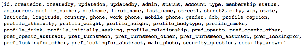

Ok, that's a lot of information. Let's start with the gender balance (I use 35 million entries, the entire database has 37 million entries or so):

gender = SQLExecute[SQLSelect["am", {"am_am_member"}, {SQLColumn[{"am_am_member", "gender"}]}, None, 
"SortingColumns" -> None, "MaxRows" -> 35000000, "Distinct" -> False, "GetAsStrings" -> False, "ShowColumnHeadings" -> True]];

We then tally this:

gendertally = Tally[Flatten@gender[[2 ;;]]][[1 ;; 2]] /. {2 -> "Male", 1 -> "Female"}
(*{{"Male", 27546956}, {"Female", 4414808}}*)

This tell us that out of the 35 million members that we analysed there are about 27.5 million male users and 4.4 million female users. Next we chart it:

PieChart[Apply[Labeled, Reverse[{{Style["Male", Large], gendertally[[1, 2]]}, 
{Style["Female", Large], gendertally[[2, 2]]}}, 2], {1}], PlotTheme -> "Business"]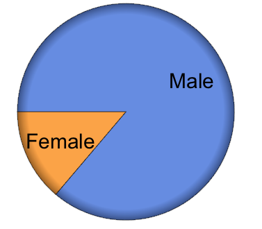

It is easy to calculate the percentages:

N@#[[2]]/Total[(Tally[Flatten@gender[[2 ;;]]][[1 ;; 2, 2]] /. {2 -> "Male", 1 -> "Female"})] & /@ 
(Tally[Flatten@gender[[2 ;;]]][[1 ;; 2]] /. {2 -> "Male", 1 -> "Female"})

Which suggestst that there are about 86.2% males and 13.8% females in this subsample of 35000000 entries (alltogether there are slighty more than 35 million entries in the databse). Let's have a look at the dates of birth - this time I will choose a 2 million subset.

dob = SQLExecute[SQLSelect["am", {"am_am_member"}, {SQLColumn[{"am_am_member", "dob"}], 
SQLColumn[{"am_am_member", "gender"}]}, !SQLStringMatchQ[SQLColumn[{"am_am_member", "dob"}], "%0000-00-00%"], 
"SortingColumns" -> None, "MaxRows" -> 2000000,"Distinct" -> False, "GetAsStrings" -> False, "ShowColumnHeadings" -> True]];

We have also retrieved the gender so that we can plot histograms for each gender:

DateHistogram[{Select[dob, #[[2]] == 2 &][[All, 1, 1]], Select[dob, #[[2]] == 1 &][[All, 1, 1]]}, 130]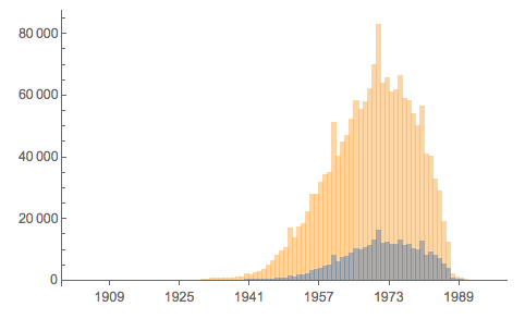

The yellow histogram shows the males and the grey the females. Let's look at gender height:

genderheight = SQLExecute[SQLSelect["am", {"am_am_member"}, {SQLColumn[{"am_am_member", "gender"}], 
SQLColumn[{"am_am_member", "profile_height"}]}, None, "SortingColumns" -> None, "MaxRows" -> 500000, 
"Distinct" -> False, "GetAsStrings" -> False, "ShowColumnHeadings" -> True]];

Here is the respective histogram by gender:

Histogram[{(Select[genderheight[[2 ;;]] /. {2 -> "Male", 1 -> "Female"}, #[[1]] == "Female" &])[[All, 2]], 
(Select[genderheight[[2 ;;]] /. {2 -> "Male", 1 -> "Female"}, #[[1]] == "Male" &])[[All, 2]]}, {120, 220, 1}, 
"Probability", AxesLabel -> {"height", "probability"}, LabelStyle -> Directive[Bold, Medium], ImageSize -> Large]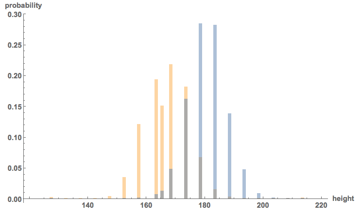

So, as we would have anticipated, women are on average slightly smaller... Nothing new here. Let's have a look at what men and women are looking for:

seekingfemale = Select[SQLExecute[SQLSelect["am", {"am_am_member"}, {SQLColumn[{"am_am_member", "gender"}],     
SQLColumn[{"am_am_member", "profile_caption"}]}, None, "SortingColumns" -> None, "MaxRows" -> 500000, 
"Distinct" -> False, "GetAsStrings" -> False, "ShowColumnHeadings" -> True]], #[[1]] == 1 &];

seekingmale = Select[SQLExecute[SQLSelect["am", {"am_am_member"}, {SQLColumn[{"am_am_member", "gender"}], 
SQLColumn[{"am_am_member", "profile_caption"}]}, None, "SortingColumns" -> None, "MaxRows" -> 500000, 
"Distinct" -> False, "GetAsStrings" -> False, "ShowColumnHeadings" -> True]], #[[1]] == 2 &];

Let's determine the important words here:

wordsfemale = DeleteStopwords[Flatten[TextWords@Select[Flatten[seekingfemale], StringQ]]]; 
wordsmale = DeleteStopwords[Flatten[TextWords@Select[Flatten[seekingmale], StringQ]]];

Here are the corresponding word-clouds:

Grid[{{"Female", "Male"}, {WordCloud[wordsfemale, IgnoreCase -> True],WordCloud[wordsmale, IgnoreCase -> True]}}, Frame -> True]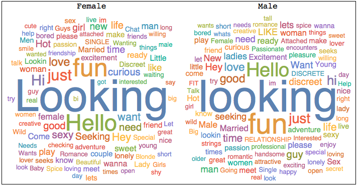

Quite clearly, very similar words come up. Does this mean that males and females are similar in what they are looking for? To illucidate this further we look at one of the entries of the database which is "pref_opento".

prefsfemale = 
  Select[SQLExecute[
    SQLSelect[
     "am", {"am_am_member"}, {SQLColumn[{"am_am_member", "gender"}], 
      SQLColumn[{"am_am_member", "pref_opento"}]}, None, 
     "SortingColumns" -> None, "MaxRows" -> 50000, 
     "Distinct" -> False, "GetAsStrings" -> False, 
     "ShowColumnHeadings" -> True]], #[[1]] == 1 &];

prefsmale = 
  Select[SQLExecute[
    SQLSelect[
     "am", {"am_am_member"}, {SQLColumn[{"am_am_member", "gender"}], 
      SQLColumn[{"am_am_member", "pref_opento"}]}, None, 
     "SortingColumns" -> None, "MaxRows" -> 50000, 
     "Distinct" -> False, "GetAsStrings" -> False, 
     "ShowColumnHeadings" -> True]], #[[1]] == 2 &];

Here's a histogram of the preferences:

Histogram[{ToExpression@(Flatten@
     StringSplit[prefsfemale[[1 ;; 50000, 2]], "|"]), 
  ToExpression@(Flatten@
     StringSplit[prefsmale[[1 ;; 50000, 2]], "|"])}, {1, 52, 
  1}, "Probability", 
 AxesLabel -> {"Number Preference", "Probability"}, 
 LabelStyle -> Directive[Bold, Medium], ImageSize -> Large]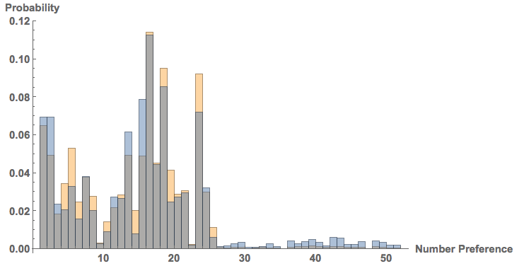

Males are blue, females orange/yellow. Each number corresponds to one -often rather explicit- preference. In the dump there is a table that allows you to interpret what these numbers mean, but for the purpose of this post, that would only be unneccessarily explicit and hence I avoid spelling out the preferences.

Let's look at the account types. It turns out that an entry "1" in the data base describes a paid-for account, whereas "2" means free.

accounttypefemale = 
  Select[SQLExecute[
    SQLSelect[
     "am", {"am_am_member"}, {SQLColumn[{"am_am_member", "gender"}], 
      SQLColumn[{"am_am_member", "account_type"}]}, None, 
     "SortingColumns" -> None, "MaxRows" -> 50000, 
     "Distinct" -> False, "GetAsStrings" -> False, 
     "ShowColumnHeadings" -> True]], #[[1]] == 1 &];
accounttypemale = 
  Select[SQLExecute[
    SQLSelect[
     "am", {"am_am_member"}, {SQLColumn[{"am_am_member", "gender"}], 
      SQLColumn[{"am_am_member", "account_type"}]}, None, 
     "SortingColumns" -> None, "MaxRows" -> 50000, 
     "Distinct" -> False, "GetAsStrings" -> False, 
     "ShowColumnHeadings" -> True]], #[[1]] == 2 &];

For female we get:

SortBy[Tally[accounttypefemale[[All, 2]]], #[[1]] &] /. {1 -> "Paid", 2 -> "Free"}
(*{{"Paid", 4798}, {"Free", 868}}*)

For male we get:

SortBy[Tally[accounttypemale[[All, 2]]], #[[1]] &] /. {1 -> "Paid", 2 -> "Free"}
(*{{"Paid", 44307}, {"Free", 22}}*)

Virtually all males have a paid for account. That is interesting. Let's have a look at when the accounts were created:

createdonfemale = 
  Select[SQLExecute[
    SQLSelect[
     "am", {"am_am_member"}, {SQLColumn[{"am_am_member", "gender"}], 
      SQLColumn[{"am_am_member", "createdon"}]}, ! 
      SQLStringMatchQ[SQLColumn[{"am_am_member", "createdon"}], 
       "%0000-00-00 00:00:00%"], "SortingColumns" -> None, 
     "MaxRows" -> 1000000, "Distinct" -> False, 
     "GetAsStrings" -> False, 
     "ShowColumnHeadings" -> True]], #[[1]] == 1 &];
createdonmale = 
  Select[SQLExecute[
    SQLSelect[
     "am", {"am_am_member"}, {SQLColumn[{"am_am_member", "gender"}], 
      SQLColumn[{"am_am_member", "createdon"}]}, ! 
      SQLStringMatchQ[SQLColumn[{"am_am_member", "createdon"}], 
       "%0000-00-00 00:00:00%"], "SortingColumns" -> None, 
     "MaxRows" -> 1000000, "Distinct" -> False, 
     "GetAsStrings" -> False, 
     "ShowColumnHeadings" -> True]], #[[1]] == 2 &];

Here's a time line plot for the females:

TimelinePlot@createdonfemale[[1 ;; 1000, 2, 1]]

Here is the one for the males:

TimelinePlot@createdonmale[[1 ;; 1000, 2, 1]]

These plots are not very telling only show that there might be interesting information in the arrival times.

DateHistogram[{createdonmale[[;; , 2, 1]], createdonfemale[[;; , 2, 1]]}, 500, PlotRange -> {{DateObject[{2001, 1, 1}], 
DateObject[{2006, 7, 1}]}, All}, AxesLabel -> {"date", "number of registrations"}, LabelStyle -> Directive[Bold, Medium], 
ImageSize -> Large]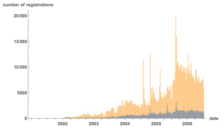

It is interesting to see that there are large peaks. Also, apart form the very beginning there are always more men to sign up then women. To study this further we can look at the differences between two arrival times; the time series is obviously not stationary, but could there be an underlying Poisson-process?

arrivaltimesfemale = 
Table[DateDifference[createdonfemale[[i, 2, 1]], createdonfemale[[i + 1, 2, 1]], Quantity[1, "Seconds"]], {i, 1, 50000}];

arrivaltimesmale = 
Table[DateDifference[createdonmale[[i, 2, 1]], createdonmale[[i + 1, 2, 1]], Quantity[1, "Seconds"]], {i, 1, 50000}];

Here are the histograms:

Grid[{{"female", 
   Histogram[QuantityMagnitude /@ arrivaltimesfemale, "Log", 
    ImageSize -> Medium]}, {"male", 
   Histogram[QuantityMagnitude /@ arrivaltimesmale, "Log", 
    ImageSize -> Medium]}}, Frame -> All]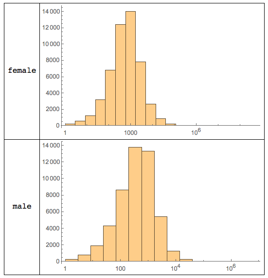

That is quite interesting. The histograms appear to be quite different. Let's check what type of distributions Wolfram Language believes this to be:

FindDistribution[Select[(QuantityMagnitude /@ arrivaltimesfemale[[1 ;; 2000]]), # > 0 &], 3]
(*{MixtureDistribution[{0.921977, 0.0780234}, {LogNormalDistribution[7.64884, 1.99741], GammaDistribution[3.03315, 11677.4]}], 
 MixtureDistribution[{0.938047, 0.0619529}, {LogNormalDistribution[7.66677, 1.97593], LogNormalDistribution[10.7177, 0.441292]}], 
 LogNormalDistribution[7.84679, 2.04246]}*)

and for the males:

FindDistribution[Select[(QuantityMagnitude /@ arrivaltimesmale[[1 ;; 2000]]), # > 0 &], 3]
(*{ParetoDistribution[3564.88, 2.03308, 1.08316, 1.00978], LogNormalDistribution[7.22247, 1.7025], FrechetDistribution[1.03896, 1219.71, -317.249]}*)

Next, we look at the geo-spacial distribution. Luckily, the database comes with GPS coordinates. (It also contains the address of the member.) I will not display any GPS coordinates in this post, as to not identify individuals. Instead I will display points on a world-wide map and a density distribution for the United States.

geocordsfull = SQLExecute[
   SQLSelect["am", {"am_am_member"}, {SQLColumn[{"am_am_member", "latitude"}], SQLColumn[{"am_am_member", "longitude"}]}, None, 
    "SortingColumns" -> None, "Distinct" -> False, "MaxRows" -> 1000000, "GetAsStrings" -> False, "ShowColumnHeadings" -> True]];

First the global distribution of the first 10000 entries:

GeoListPlot[GeoPosition /@ (DeleteCases[RandomChoice[geocordsfull, 10000], {0., 0.}]), 
GeoBackground -> "ReliefMap", GeoCenter -> GeoPosition[{0, 0}], ImageSize -> Large]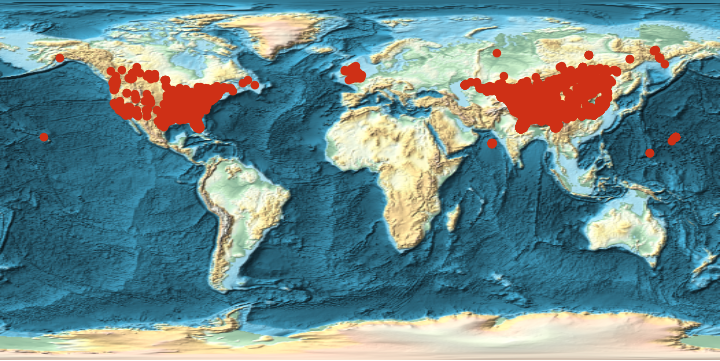

Ok, next the plot for the US. We first select particular geocoordinates, then calculate a density, and then plot it over the map of the United States:

adulterercoordsusa = Select[RandomChoice[geocordsfull, 20000], (24.9382 < #[[1]] && #[[1]] < 49.37 && -67 > #[[2]] && #[[2]] > -124) &];
adultererDensityDistribution = SmoothKernelDistribution[adulterercoordsusa, "SheatherJones"];

The final stage is to plot the density and the map of the US:

cplot = ContourPlot[PDF[adultererDensityDistribution, {y, x}], 
   Evaluate@
    Flatten[{x, {#[[1, 1, 2]], #[[2, 1, 2]]} &@
       GeoBoundingBox[Entity["Country", "UnitedStates"]]}], 
   Evaluate@
    Flatten[{y, {#[[1, 1, 1]], #[[2, 1, 1]]} &@
       GeoBoundingBox[Entity["Country", "UnitedStates"]]}], 
   ColorFunction -> "Rainbow", Frame -> False, 
   PlotRange -> {0, 0.027}, Contours -> 205, MaxRecursion -> 2, 
   ColorFunction -> ColorData["TemperatureMap"], 
   PlotRangePadding -> 0, ContourStyle -> None];
GeoGraphics[{GeoStyling[{"GeoImage", cplot}], 
  Polygon[Entity["Country", "UnitedStates"]], Black, Opacity[1], 
  PointSize[0.0015], Point[Reverse /@ adulterercoordsusa]}, 
 GeoRange -> Entity["Country", "UnitedStates"], ImageSize -> Large]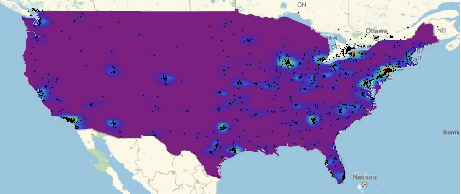

There is much more interesting stuff in the am database, but let's proceed to the aminno database.

CloseSQLConnection[am];
OpenSQLConnection["aminno", "Name" -> "aminno_member", "Password" -> "loyaltyandfidelity"]

Again as above you can use the

DatabaseExplorer[]

to make the database available to Mathematica. Let's look at the IP addresses that were used for signing up:

TableForm@(Reverse@
    SortBy[Tally[
      DeleteCases[
        Flatten[SQLExecute[
          SQLSelect[
           "aminno", {"aminno_member"}, {SQLColumn[{"aminno_member", 
              "signupip"}]}, None, "SortingColumns" -> None, 
           "MaxRows" -> 1000000, "Timeout" -> 10, "Distinct" -> False,
            "GetAsStrings" -> False, "ShowColumnHeadings" -> True]]], 
        ""][[2 ;;]]], #[[2]] &])[[1 ;; 25]]

This gives:

The interesting bit is that it contains the ip-address 127.0.0.1 which is "localhost". The first entry is an AOL address for example. Now we can ask how many people have certain email domains. First we get all email addresses. I will not display individual email addresses to protect individuals.

emails = DeleteCases[(Flatten@SQLExecute[SQLSelect["aminno", {"aminno_member_email"}, 
{SQLColumn[{"aminno_member_email", "email"}]}, None,  "SortingColumns" -> None, "MaxRows" -> 10000000, 
"Timeout" -> 100, "Distinct" -> False, "GetAsStrings" -> False, "ShowColumnHeadings" -> True]])[[2 ;;]], ""];

We can count how many have a ".mil" address.

Length[Select[emails, StringMatchQ[#, __ ~~ ".mil"] &]]
(*3588*)

This means that for the entire 37 million entries we would expect about 13276 ".mil"-addresses. This is the number of uk govermental addresses:

Length[Select[emails, StringMatchQ[#, __ ~~ ".gov.uk"] &]]
(*34*)

There is another entry in the database which is called bcmaillast_time. It gives the time when the member checked the email last time. If the member never checked the email there will be all zeros in that entry. We therefore look at all females with non-zeros at that entry:

emailactivity = (SQLExecute[SQLSelect["aminno", {"aminno_member"}, 
{SQLColumn[{"aminno_member", "bc_mail_last_time"}],SQLColumn[{"aminno_member", "gender"}]},                 
!SQLStringMatchQ[SQLColumn[{"aminno_member", "bc_mail_last_time"}], 
"%0000-00-00 00:00:00%"], "SortingColumns" -> None, "MaxRows" -> 2000000, "Timeout" -> 1100, 
"Distinct" -> False, "GetAsStrings" -> False, "ShowColumnHeadings" -> True]][[2 ;;]]);

So how many of the first 2000000 entries in the data base, i.e. people, were female:

Length@(Select[emailactivity, #[[2]] == 1 &][[All, 1, 1]])
(*254*)

Ups, that frighteningly low! the remainder are men:

(Length@Select[emailactivity, #[[2]] == 2 &][[All, 1, 1]])
(*1999746*)

Wow, that means that there are very few active women indeed. If I want to analyse the entire database, Java runs out of heaps-space. Luckily, there is a command to fix that:

<< JLink`;
InstallJava[];
ReinstallJava[CommandLine -> "java", JVMArguments -> "-Xmx16384m"]

Nice, now we've got all we need.

emailactivity = (SQLExecute[
     SQLSelect[
      "aminno", {"aminno_member"}, {SQLColumn[{"aminno_member", 
         "bc_mail_last_time"}], 
       SQLColumn[{"aminno_member", "gender"}]}, ! 
       SQLStringMatchQ[
        SQLColumn[{"aminno_member", "bc_mail_last_time"}], 
        "%0000-00-00 00:00:00%"], "SortingColumns" -> None, 
      "MaxRows" -> 21000000, "Timeout" -> 1500, "Distinct" -> False, 
      "GetAsStrings" -> False, "ShowColumnHeadings" -> True]][[2 ;;]]);

That last command lists up to 21 million entries that do not have zeros in the last reply, i.e. "sign-of-life" field. In a moment we will see that that covers all people, who show at least some activity beyond registration. Out of these there are

Length@(Select[emailactivity, #[[2]] == 1 &][[All, 1, 1]])
(*1492*)

1492 females only!!! And there are:

Length@(Select[emailactivity, #[[2]] == 2 &][[All, 1, 1]])
(*20269675*)

20269675 males. Note that both numbers add up to less than 21 million, i.e. we have extracted all at least briefly active members. This means that of over 20 million users who actually used the system, beyond registration, only 1492 were women. That corresponds to:

100*1492/(1492 + 20269675) // N

i.e. , 0.0074% women. This suggests that many men have paid to meet women, who were not (active) in the system.

This analysis is far from complete. It just shows what can be achieved with Mathematica on a standard laptop. The dataset has many different types of data. I think that this analysis could be considered as a first step towards "big-data". Wolfram Language is quite capable to analyse rather large datasets even on standard home equipment. It is a really nice tool for big data, which is not only large, but also contains very heterogenous data. Wolfram Language functions for text analysis, efficient algorithms to perform operations on large data sets, and the curated data have all proven to be useful. There are many more things that Wolfram Language can help to extract from this particular database, but this post is already far to long, for which I apologise. If there is any interest for this kind of analysis, or if there are questions/suggestions about what else to do with the data, I will be happy to post that, as long as it does not disclose any personal information of the people involved.

Cheers,

Marco